Neural Networks

Imagine you’re teaching a child to recognize handwritten numbers from 0 to 9. At first, they might struggle, but with practice, by seeing many examples and receiving feedback, they learn to recognize patterns. Neural networks (NNs) work in a similar way, learning from examples to make predictions.

Let’s say we want a computer program to read handwritten numbers. The process happens in several steps:

1. Training with Examples: We show the program thousands of handwritten numbers with the correct labels (e.g., “This is a 5”).
2. Detecting Features: The program first identifies basic shapes like lines and curves. For example, a “3” has two curves, while a “7” has a straight top and a diagonal line.
3. Making a Guess: After analyzing the features, the program makes a prediction (e.g., “This looks like a 3”).
4. Checking and Learning: If the guess is wrong, let’s say it thought a “3” was an “8”, the program corrects itself by adjusting its internal settings. It learns which shapes that matter most and improves over time.

The more examples it processes, the better it becomes at recognizing numbers, just like a child learning to read handwriting.

How Neural Networks Work

Neural networks are inspired by the human brain. Just as our brain has neurons that process information, NNs have layers of artificial neurons that analyze data step by step. These layers are:

• Input Layer: Receives information (e.g., a picture of a handwritten number).
• Hidden Layers: Processes the information, identifying patterns and relationships.
• Output Layer: Produces the final decision (e.g., “This is a 7”).

Each connection between neurons has a “weight,” which determines its importance. Initially, these weights are random, but as the program trains, they are adjusted to improve accuracy.

A Real-Life Example: Sorting Fruits

Imagine you’re sorting apples and oranges with a blindfold on. At first, you might guess based on size or texture, making mistakes. But if someone corrects you each time, you’ll eventually learn that apples are smoother and rounder, while oranges have a rougher texture.

Similarly, an Neural network starts with guesses but improves through feedback. Over time, it becomes highly accurate in distinguishing between different objects.

---

The Evolution of Neural Networks

Scientists have been developing Neural networks for decades:

• 1958: Frank Rosenblatt created the Perceptron, the first ANN algorithm that could learn basic patterns.
• 1960: Bernard Widrow designed a network that could predict patterns in phone signals, helping improve communication technology.
• 1974: Paul Werbos suggested using neural networks for problem-solving, leading to more advanced learning systems.
• 1986: Researchers popularized the backpropagation algorithm, allowing networks to learn from mistakes more effectively.

Training Neural Networks with Backpropagation

For decades, backpropagation has been the backbone of Neural networks, playing a crucial role in training these systems to recognize patterns, classify data, and make predictions. As one of the most fundamental algorithms in machine learning, backpropagation has enabled significant advancements in areas such as image recognition, speech processing, and financial forecasting. While newer techniques have begun to surpass backpropagation in certain applications, understanding this algorithm remains essential to grasping the foundations of deep learning.

Understanding Backpropagation

Backpropagation, short for “backward propagation of errors,” is a supervised learning algorithm used to train Neural networks. It works by adjusting the weights of connections between neurons based on the difference between predicted and actual outputs. This iterative process enables the network to improve its accuracy over time, gradually learning the best set of parameters to minimize errors.

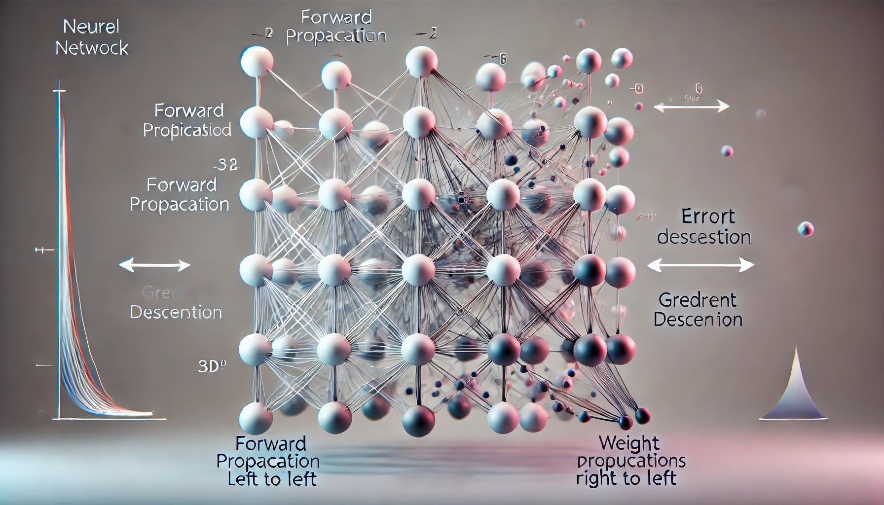
The process of backpropagation involves two key steps: forward propagation and backward propagation. During forward propagation, input data is passed through multiple layers of neurons, each performing mathematical transformations, to produce an output. If this output does not match the expected result, the error is computed. The backward propagation step then calculates how this error should be distributed across the network and adjusts the weights accordingly using an optimization technique known as gradient descent.

Gradient Descent: The Learning Mechanism

At the core of backpropagation lies gradient descent, an optimization algorithm that helps the neural network adjust its weights in the right direction to minimize error. Gradient descent can be understood by comparing it to hiking down a mountain in thick fog. If you cannot see the bottom, you rely on sensing the slope beneath your feet. Moving in the direction where the ground declines ensures that you eventually reach the lowest point. Similarly, gradient descent follows the slope of the error function, making small, calculated weight adjustments to gradually improve the network’s accuracy. Backpropagation is the learning mechanism that allows a neural network to improve over time. It does this by adjusting its internal connections (weights) based on the mistakes it makes.

Imagine you’re teaching a child to recognize numbers, but instead of telling them outright, you only give feedback when they get it wrong. Over time, they learn from their mistakes and improve. Backpropagation works in a similar way. Let’s break it down into five simple steps:

Step 1: Forward Pass – Making a Prediction

At first, the neural network makes a guess based on what it has learned so far.

• Imagine the post office is using a neural network to read handwritten ZIP codes. A new envelope arrives, and the system scans the number “23527.” However, the network mistakenly reads it as “73527” because it confuses the “2” with a “7.”
• The neural network has input layers (which take the pixel data from the image), hidden layers (which process the patterns), and an output layer (which predicts the numbers).
• Each neuron in the network has a weight that determines how much importance it gives to different parts of the image. The network processes the image, applies these weights, and outputs 73527 instead of 23527.

Step 2: Compute the Error (Loss Function)

Now, we need to measure how wrong the network’s prediction was.

The system compares the predicted ZIP code (73527) with the correct one (23527).
It calculates an error value using a formula called a loss function (such as Mean Squared Error or Cross-Entropy Loss).
The bigger the error, the more the system needs to adjust its internal weights.

Think of it like a teacher grading a test. If a student gets many answers wrong, they need more practice on those topics.

Step 3: Backward Pass – Tracing Back the Mistake

Now, the system needs to figure out which parts of the network contributed the most to the mistake.

• The network moves backward from the output layer (wrong ZIP code) toward the input layer.
• It assigns blame to each neuron based on how much it contributed to the error.
• If certain neurons mistakenly thought a “2” looked like a “7,” their weights need to be adjusted to avoid making the same mistake again.

Step 4: Adjusting Weights Using Gradient Descent

Now that we know which neurons caused the mistake, we need to fix them. This is where gradient descent comes in.

• Gradient descent is like a GPS for finding the best weight values.
•  It calculates the direction and size of changes needed to minimize the error.
•  The network updates the weights slightly in the direction that reduces the error.

 Analogy: Imagine you’re walking downhill in the dark (minimizing the error).

• If the slope is steep, you take big steps.
• If it’s shallow, you take smaller steps.
• The goal is to reach the bottom (where the error is lowest).

The network keeps adjusting the weights little by little until it gets closer to the correct ZIP code.

Step 5: Repeat Until the Network Learns

 The process repeats for thousands or millions of training examples.
 Each time, the neural network gets a little better at recognizing handwritten numbers.
 Over time, it becomes highly accurate and makes fewer mistakes.

Why Is Backpropagation So Powerful?

• It makes learning efficient – Instead of randomly changing weights, the network makes targeted improvements.
• It enables deep learning – Backpropagation allows networks with many layers (deep networks) to learn complex patterns.
• It automates feature learning – Instead of manually defining what a “2” or “7” looks like, the network learns on its own.

Why Backpropagation Was the Standard for Decades

Backpropagation became the dominant training algorithm for neural networks due to its efficiency, simplicity, and versatility. In the 1980s, researchers such as Rumelhart, and Williams rediscovered and popularized the backpropagation algorithm, making it a practical tool for training multilayer neural networks. Before its widespread use, training deep networks was nearly impossible because there was no effective method to adjust weights in deeper layers. Backpropagation solved this problem by providing a systematic way to update weights layer by layer. Over time, backpropagation has been used in various domains.

The Shift Toward Newer Techniques

Despite its historical success, backpropagation has certain limitations. It struggles with training very deep neural networks due to issues like vanishing gradients, where updates become too small to be effective in deep layers. Additionally, backpropagation requires large labeled datasets and significant computational power. As a result, researchers have developed more advanced training methods and architectures.

For instance, convolutional neural networks (CNNs) have revolutionized image processing by automatically detecting hierarchical features, reducing the need for extensive manual feature engineering. Similarly, transformers have transformed natural language processing (NLP) by enabling models to capture long-range dependencies and contextual relationships more effectively than traditional recurrent networks. Techniques like self-attention and pretraining on vast unlabeled datasets have significantly improved learning efficiency and accuracy in tasks like language translation and text generation.

These advancements address some of backpropagation’s inefficiencies, making modern neural networks more scalable, adaptable, and powerful across diverse applications.

Conclusion

Backpropagation remains a cornerstone of artificial intelligence, providing the foundation for many neural network applications. By using gradient descent to iteratively improve performance, this algorithm has enabled machines to learn from mistakes and make accurate predictions. While more advanced techniques are emerging, understanding backpropagation is essential for anyone interested in the inner workings of AI. Whether in postal services, healthcare, or financial markets, the impact of backpropagation continues to shape the future of machine learning and artificial intelligence.